Choice of Loss in Proximal Policy Optimization

The full code for this project is available in this kaggle notebook.

I’ve been self-studying machine learning recently, and I’m having a lot of fun. It’s been a long time since I’ve had the opportunity to systematically digest the basics of a new field. High quality resources for this material are abundant (e.g. Andrej Karpathy’s videos), and in a meta twist the chatbots themselves are incredibly useful for learning the technology behind chatbots. This has of course been great for my learning rate, but spoon-feeding eventually makes me a bit restless. I was excited, then, to finally engage with a question that chatbots and google-foo couldn’t answer. My experiments for it are the subject of this blog post.

For the past couple of weeks I’ve been studying reinforcement learning (RL) by going through OpenAI Spinning Up and playing around with implementations of some standard RL algorithms for the CartPole-v1 environment in the gymnasium package. This environment simulates a pole with one end attached to a cart. You control the cart, and your goal is to keep the pole balanced above the cart. A visualization of a well-trained model can be found here.

The state space consists of your position, velocity, angle, and angular velocity, represented as floats. The action space just consists of 0 and 1, corresponding to left and right. The reward is the number of time steps elapsed. The episode is either terminated when the angle exceeds 24 degrees, or truncated once the reward reaches 500.

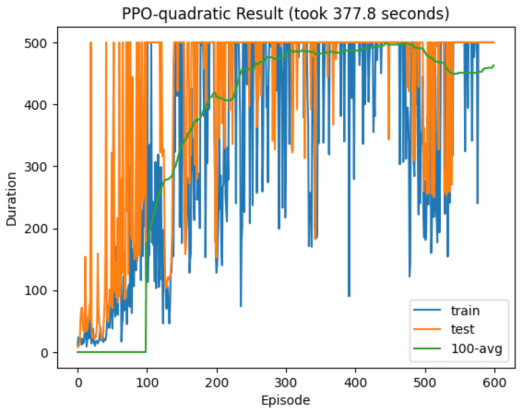
The algorithms I’ve played with so far are tabular Q-learning (with a discretized version of the environment), deep Q-network (DQN), vanilla policy gradient (VPG), and finally Proximal Policy Optimization (PPO). There was a clear hierarchy of performance, with PPO alone at the top. It dominated in both sample efficiency and wall-clock time. Admittedly I didn’t try very hard to optimize the other models’ hyperparameters, but part of the advantage of PPO is that you don’t need to work as hard to get good performance.

Here are some typical runs from each algorithm:

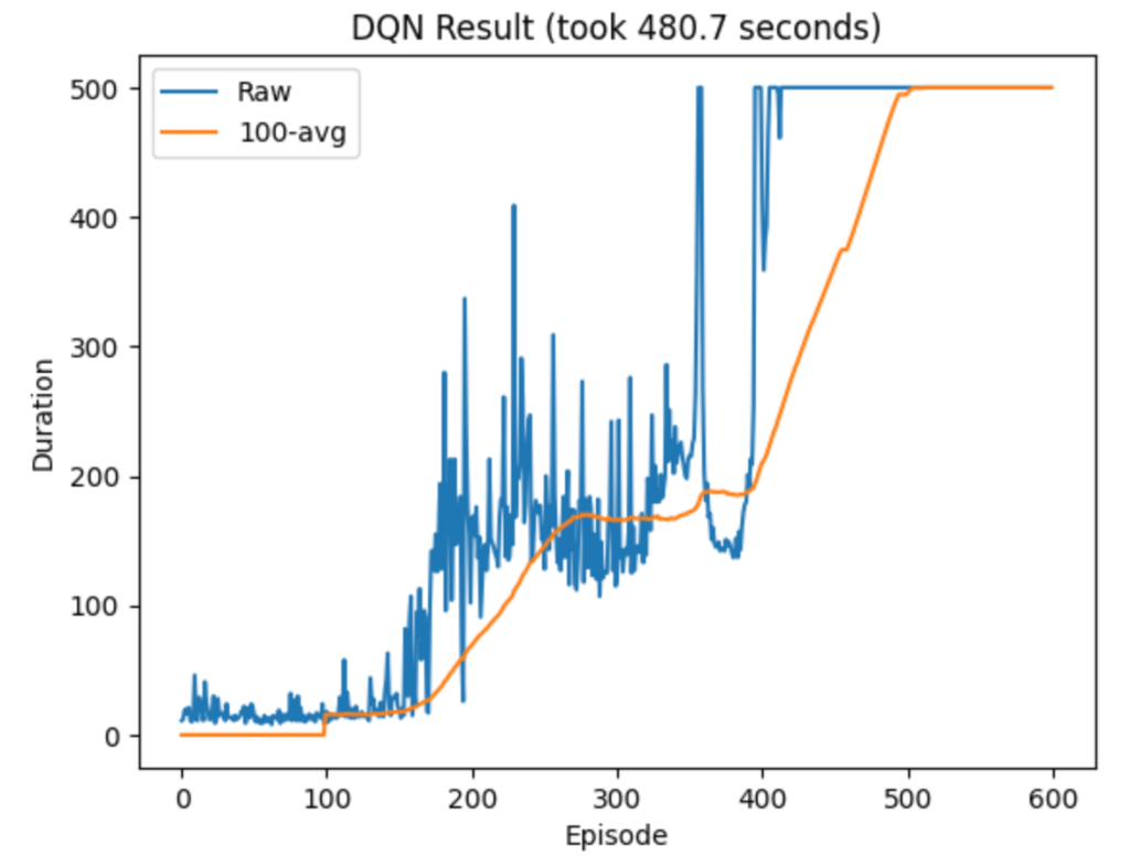
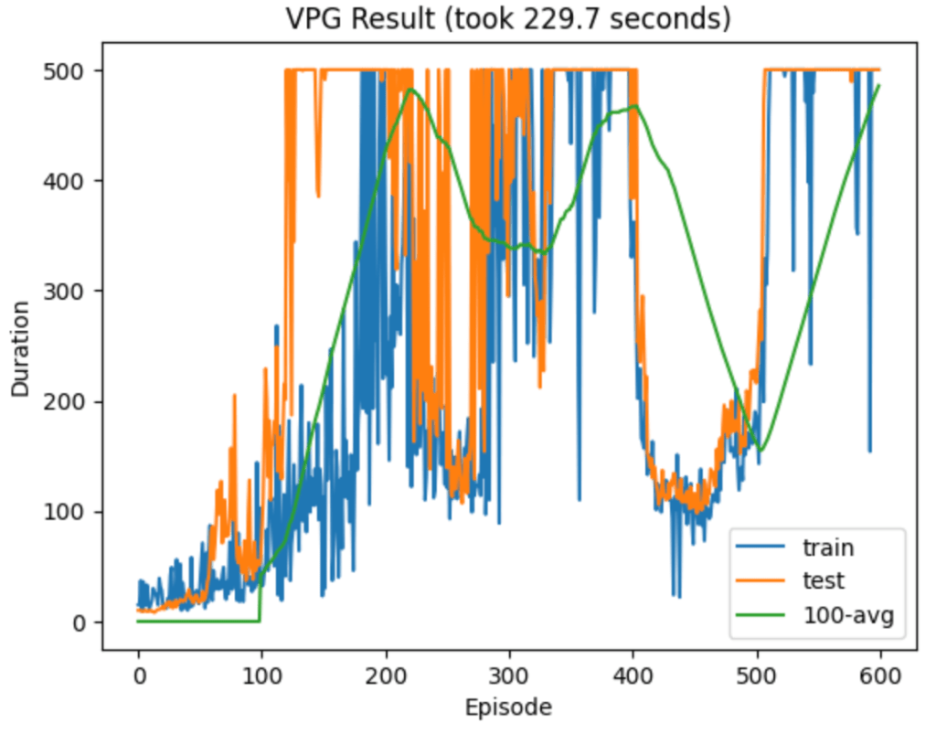
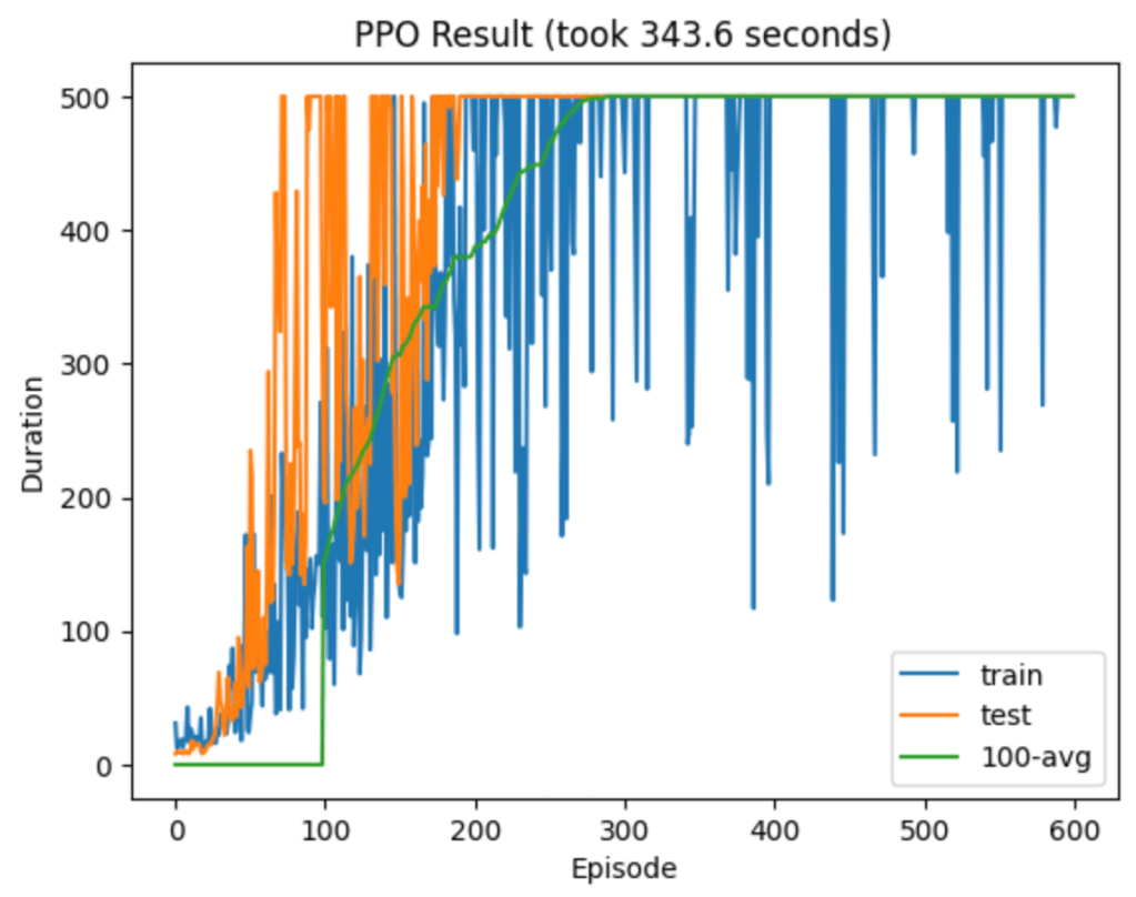
The dominance of PPO got me wondering which aspects contribute most to its success. The main differences from VPG are that it takes multiple optimization steps after each episode, it uses a different surrogate loss, and it clips this loss if the new policy strays too far from the previous one. (I’ll use “loss” and “objective” interchangeably, even though the latter is more technically correct here.)

Writing $J[\pi_\theta] = E_{\pi_\theta}[R[\tau]]$ for the total expected reward of an episode trajectory $\tau$ sampled from the policy $\pi_\theta$ , the gradient is

$\nabla_\theta J[\pi_\theta] = E_{\pi_\theta}\big[ R[\tau] \nabla_\theta \log \pi_\theta[\tau] \big]$ ,

where $\nabla_\theta \log \pi_\theta[\tau]$ comes from the gradient hitting the probability measure in the expectation. Usually one works in terms of the advantage $A_t$ at each time step, rather than the total reward $R[\tau]$ . The gradient then reads

$\nabla_\theta J[\pi_\theta] = \sum_t E_{\pi_\theta}\big[ A_t \nabla_\theta \log \pi_{\theta, t} \big]$

where I’m using $\pi_{\theta, t}$ as shorthand for the probability $\pi_\theta(a_t, s_t)$ of choosing action $a_t$ in state $s_t$ . If we distinguish between the “old” parameters $\theta_0$ (before training on the most recent episode) and the current parameters $\theta$ , then the policy gradient can be rewritten as the gradient of a convenient loss:

$L^{PG}(\theta; \theta_0) \equiv \sum_t E_{\pi_{\theta_0}} \big[ A_t \log \pi_{\theta, t} \big]$ .

The policy gradient coincides with the gradient of $L^{PG}$ when $\theta=\theta_0$ , or in other words

$(\nabla_\theta L^{PG})|_{\theta = \theta_0} = \nabla_\theta J[\pi_\theta]$ .

Introductory policy gradient discussions emphasize repeatedly that this should not be misinterpreted as saying that $L^{PG}$ approximates $J[\pi_\theta]$ . As soon as $\theta \ne \theta_0$ , the gradients are no longer equal.

With this warning fresh in my mind, it seemed strange that PPO continues to use a surrogate loss even after $\theta \ne \theta_0$ . My first thought was that maybe PPO’s choice of surrogate loss was somehow better than $L^{PG}$ . For reference, PPO uses

$L^{PPO}(\theta; \theta_0) \equiv \sum_t E_{\pi_{\theta_0}} \big[ \frac{\pi_{\theta,t}}{\pi_{\theta_0, t}} A_t \big]$ ,

where $\pi_{\theta,t} / \pi_{\theta_0,t}$ is known as the policy ratio. But after reading the original PPO and TRPO papers from Schulman et al. to see where this loss came from, my sense is that it is basically a historical quirk stemming from the particular math theorems that motivate TRPO.

First Hypothesis

To test this hypothesis, I modified the PPO algorithm to use $L^{PG}$ instead of $L^{PPO}$ and compared its performance with PPO for the CartPole-v1 environment. In my initial PPO algorithm (from a nice tutorial by Arun Nanda) the function calculating the surrogate loss is:

def calculate_surrogate_loss(
        actions_log_probability_old,
        actions_log_probability_new,
        epsilon,
        advantages):
    advantages = advantages.detach()
    policy_ratio = (
            actions_log_probability_new - actions_log_probability_old
            ).exp()
    surrogate_loss_1 = policy_ratio * advantages
    surrogate_loss_2 = torch.clamp(
            policy_ratio, min=1.0-epsilon, max=1.0+epsilon
            ) * advantages
    surrogate_loss = torch.min(surrogate_loss_1, surrogate_loss_2)
    return surrogate_loss

The inputs here are the clipping parameter $\epsilon$ , the advantages $A_t$ , and the old and new log probabilities $\log\pi_{\theta_0,t}$ and $\log\pi_{\theta, t}$ for an episode. After computing the policy ratio $\pi_{\theta,t} / \pi_{\theta_0,t}$ , the function computes the surrogate loss’s contribution from each time $t$ , clipping contributions where the policy ratio is outside of $1\pm\epsilon$ . My modified function is:

def calculate_surrogate_loss(
        actions_log_probability_old,
        actions_log_probability_new,
        epsilon,
        advantages):
    advantages = advantages.detach()
    surrogate_loss_1 = actions_log_probability_new * advantages
    clamped_log_probs = torch.clamp(actions_log_probability_new,
                             actions_log_probability_old + np.log(1-epsilon),
                             actions_log_probability_old + np.log(1+epsilon)
                             )
    surrogate_loss_2 = clamped_log_probs * advantages
    surrogate_loss = torch.min(surrogate_loss_1, surrogate_loss_2)
    
    return surrogate_loss

This is very similar, but it uses $\log\pi_{\theta,t}$ in the loss instead of the policy ratio. It clips $\log\pi_{\theta,t}$ based on $\log\pi_{\theta_0,t} + \log(1\pm\epsilon)$ , which is equivalent to clipping the policy ratio on $1 \pm \epsilon$ .

I found my modified PPO algorithm’s test performance to be comparably excellent to the original version, although for some reason its training performance seemed noisier. Here is a typical run from the modified version:

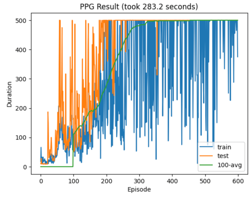
After a bit more searching around online, I actually did find a paper by Gyun et al. answering this exact question. They too modified PPO to use $L^{PG}$ , and they called their algorithm Proximal Policy Gradient (PPG). They tested it on several environments including Ant, HalfCheetah, Hopper, and Walker2d, which are more challenging than CartPole. They found that PPG performs comparably to PPO in all cases.

This is not too surprising considering that the two losses are related (up to a constant shift) by simply replacing the policy ratio with its log, and $\log x$ has unit slope at $x=1$ . Although the slopes of $x$ and $\log x$ begin to differ dramatically when $x$ is small, clipping shields us from this regime.

Second Hypothesis

This was a nice confirmation of my first hypothesis, but a mystery still remained. How was it possible that PPO and its modification PPG performed so well despite “misusing” their surrogate losses by continuing to use them after $\theta \ne \theta_0$ ? Since $L^{PG}$ and $L^{PPO}$ have the same gradient at $\theta = \theta_0$ but differ at higher orders in $\theta - \theta_0$ , I formed the hypothesis that PPO is rather insensitive to these higher order differences, and its main innovation is just squeezing more juice from the original gradient at $\theta=\theta_0$ without straying too far from the old policy (thanks to clipping). In other words, my hypothesis was that truncating $L^{PPO}$ at first order in $\theta - \theta_0$ would not affect performance (as long as we still clip based on the full policy ratio).

I found this truncation a bit tricky to implement. Initially I hoped that I could just compute the loss once per episode, at the start of the optimization loop when $\theta=\theta_0$ , and update the clipping but not the underlying loss at each optimization step. I tried using retain_graph=True in my loss.backward() calls, and making sure not to accidentally overwrite my loss, but eventually I realized that the loss.backward() call inevitably depends on the parameter values themselves, so updating them will always break it.

I got around this by maintaining an auxiliary copy of the policy net, whose parameters I’ll denote by $\theta_{\rm aux}$ . I kept $\theta=\theta_0$ throughout the training loop, instead updating $\theta_{\rm aux}$ as follows. At each optimization step I computed $\theta$ ‘s gradient, clipped with respect to the auxiliary policy ratio $\pi_{\theta_{\rm aux},t}/\pi_{\theta_0,t}$ , and then I manually passed p.grad for ${\rm p} \in \theta$ to p.grad for ${\rm p} \in \theta_{\rm aux}$ . Then I used this gradient to update $\theta_{\rm aux}$ . Only after the optimization loop was complete did I update $\theta$ to match $\theta_{\rm aux}$ using load_state_dict(). In this way the net effect after the optimization loop was as if $\theta$ had been updated at each step with the clipped, linear-truncated version of $L^{PPO}$ , as desired.

In terms of actual code, the changes were to the surrogate loss function and the optimization loop. My new surrogate loss function reads

def calculate_surrogate_loss(
        actions_log_probability_old,
        actions_log_probability_new,
        actions_log_probability_aux,
        epsilon,
        advantages):
    advantages = advantages.detach()
    policy_ratio_new = (
            actions_log_probability_new - actions_log_probability_old
            ).exp()
    policy_ratio_aux = (
            actions_log_probability_aux - actions_log_probability_old
            ).exp()
    # Implement clipping with mask instead of min
    # Technically this objective differs by a constant, but it has the same grad
    # Mask is true where the loss is NOT clipped
    mask = ((advantages < 0) & (1-epsilon < policy_ratio_aux)) | ((advantages > 0) & (policy_ratio_aux < 1+epsilon))
    surrogate_loss = (policy_ratio_new * advantages).masked_fill(~mask, 0)
    return surrogate_loss

I added the argument actions_log_probability_aux (corresponding to $\theta_{\rm aux}$ ), which is used along with actions_log_probability_old (corresponding to $\theta_0$ ) to compute a mask that tells us how to clip the loss. The underlying loss itself is computed from actions_log_probability_new (corresponding to $\theta$ ). The optimization loop code reads

for _ in range(ppo_steps):
    # Get new log prob of actions for all input states
    action_pred, value_pred = agent(states)
    value_pred = value_pred.squeeze(-1)
    action_prob = f.softmax(action_pred, dim=-1)
    probability_distribution_new = distributions.Categorical(action_prob)
    entropy = probability_distribution_new.entropy()
    # Estimate new log probabilities using old actions
    actions_log_probability_new = probability_distribution_new.log_prob(actions)

    # I added this code for the auxiliary net
    # Get aux log prob of actions for all input states
    action_pred_aux, value_pred_aux = agent_aux(states)
    value_pred_aux = value_pred_aux.squeeze(-1)
    action_prob_aux = f.softmax(action_pred_aux, dim=-1)
    probability_distribution_aux = distributions.Categorical(action_prob_aux)
    entropy_aux = probability_distribution_aux.entropy()
    # Estimate aux log probabilities using old actions
    actions_log_probability_aux = probability_distribution_aux.log_prob(actions)
    actions_log_probability_aux = actions_log_probability_aux.detach()            

    # Use my new version of surrogate loss
    surrogate_loss = calculate_surrogate_loss(
            actions_log_probability_old,
            actions_log_probability_new,
            actions_log_probability_aux,
            epsilon,
            advantages)
    
    policy_loss, value_loss = calculate_losses(
            surrogate_loss,
            entropy,
            entropy_coefficient,
            returns,
            value_pred)

    # Compute the theta gradient
    optimizer.zero_grad()
    policy_loss.backward()
    value_loss.backward()
    # Transfer the theta gradient to theta_aux
    opt_aux.zero_grad()
    for param_src, param_aux in zip(agent.parameters(), agent_aux.parameters()):
        if param_src.grad is not None:
            param_aux.grad = param_src.grad.clone()
    # Update theta_aux
    opt_aux.step()

# Now that optimization loop is done, update theta to match theta_aux
agent.load_state_dict(agent_aux.state_dict())

Note that I never call optimizer.step(), because I don’t want to update $\theta$ inside the loop. The loop proceeds by first computing actions_log_probability_new (corresponding to $\theta$ ), which doesn’t actually change from one step to the next, and then computing actions_log_probability_aux. These are then fed into my new surrogate loss function. After calling .backward() on the resulting loss, the gradients are transferred from agent (which depends on $\theta$ ) to agent_aux (which depends on $\theta_{\rm aux}$ ), and then we update $\theta_{\rm aux}$ with opt_aux.step(). Finally, outside the optimization loop, we update $\theta$ using agent_aux’s state dict.

Below are some plots of the new model’s performance. The latter plot is more typical.

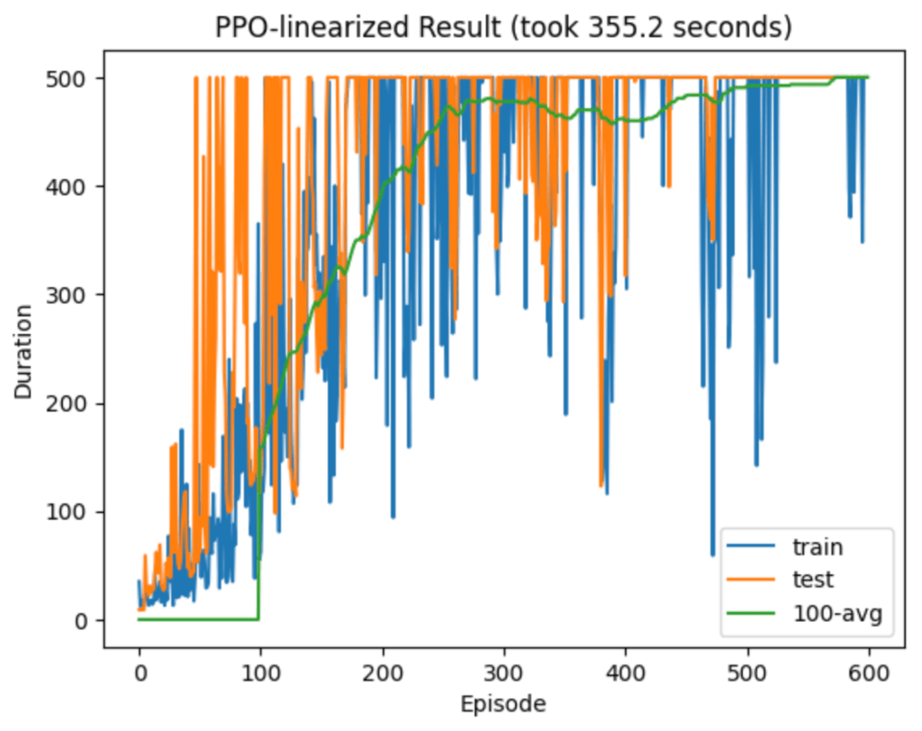
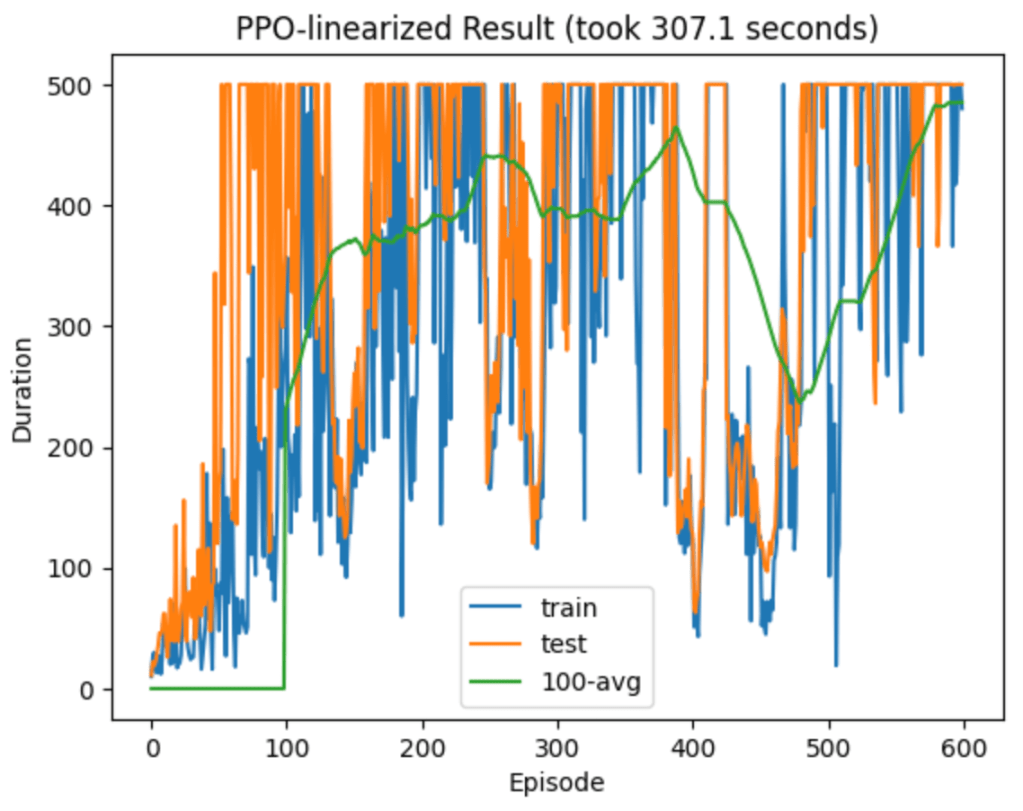
It’s noticeably worse than both PPO and PPG! It still learns quickly, but it seems prone to deep relapses into poor play. The initial learning, for the first 100 or so episodes, is still impressive and comparable to the PPO and PPG algorithms. In this regime my second hypothesis of sensitivity only to the linear part of the loss does seem plausible. But this model’s instability after attaining perfect play at least partially refutes my second hypothesis, and I don’t yet understand why it happens.

To recap, I have tested three versions of PPO using different surrogate losses $L^{PPO}$ , $L^{PPG}$ , and $L^{\rm linear}$ . These losses are identical at linear order in $\theta - \theta_0$ , but differ at second order. If PPO were only sensitive to the linear part then we would expect all three losses to perform similarly, but this was not the case. The linear-truncated loss performed worse. So PPO seems to be sensitive to second-order terms, and yet $L^{PPO}$ and $L^{PPG}$ performed similarly well despite differing at second order.

I found that truncating $L^{PPO}$ at quadratic order (implemented using torch.autograd.grad with create_graph=True) offered noticeable but meager improvement on the linear truncation. Here is a typical run:

It would be interesting to explore this further, but at this point I am getting well beyond the 80/20 rule of thumb for optimal use of one’s time. A reasonable next step would be to simultaneously track the gradients of multiple different loss types and see when they differ most, with special focus on relapses. Also, the instability after initially reaching perfect play could plausibly be mitigated by an appropriate learning rate schedule, in contrast with the constant learning rate used throughout my experiments. For now I will set these questions aside, and hopefully return to them later once I am a more experienced machine learning researcher.